Molecular modelling of crystal structures --
part 3
More advanced simulations
In this excercise, you will do quantum mechanical (QM) calculations to obtain
better atomic charges, do molecular dynamics (MD) simulations, create a
model of a crystal surface and study the interaction between a solvent and a
crystal surface.
The QM calculations can only be run when Cerius2 itself is running on the
vstofsgi.sci.kun.nl server. To get that running follow these steps:
1. If Cerius2 is still running, quit it.
2. In the terminal window, type ssh -X vstofsgi.sci.kun.nl followed by Enter and give your password
when asked for it.
3. At the command prompt, type c42 followed by Enter to start Cerius2 again. Now the Cerius2 program
is running on the vstofsgi.sci.kun.nl server.
QM calculations
The Dreiding force field (and others as well) is
intended for use in combination with atomic charges derived from the
electrostatic potential (ESP charges). A good way to calculate the ESP is
by doing a QM calculation on the molecule, from which the wave function, and
thereby the electron density canbe obtained. The electrostatic potential
follows directly from the electron density.
the Gaussian interface
One program to do QM calculations is Gaussian94. Gaussian94 has no GUI
(Graphical User Interface) itself, but Cerius2 does contain a graphical
interface to this program. It can be found under the QUANTUM 1
card on the card deck. Here, we will calculate ESP charges for
4-hydroxy- 2-thiophenecarbonitrile (C5SNOH3), also known as CSP99-2, and shown below.
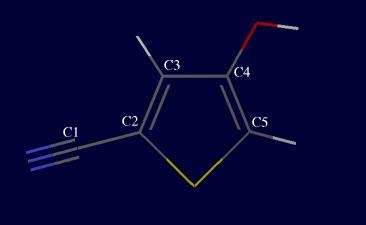
Draw the molecule, and optimize it using Dreiding. The -OH group has two
possible conformations, which have (C3-C4-O-H)-torsion angles of 0 and 180
degrees respectively. You can measure torsion angles (and other
geometry-related quantities) via the Geometry | Measurements...
menu in the main Visualizer window.
Take the conformation that has a torsion angle of 180 degrees.
Go to QUANTUM 1 on the card deck, and select GAUSSIAN.
Click Run to get the window that allows to set the parameters for
the calculation. This window is shown here.
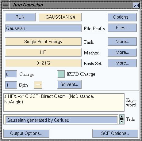
Gaussian has had several releases, and we will use the 1994
release, aptly named "Gaussian94". By default, Cerius will look for Gaussian92,
so start by selecting GAUSSIAN 94, in the top of the window.
structure optimization and ESP charge calculation
We want to do the ESP calculation on the optimized geometry of the molecule.
The molecule has already been optimized with Dreiding, which brings it close
to the optimized QM geometry. We could have used the sketched molecule right
away in Gaussian (i.e. without the MM optimization), but the QM calculations
take a lot of time, so it is more efficient to use a quick method to arrive
at a geometry that is close to what it should be, ergo molecular mechanics.
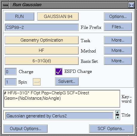
Now set up the QM calculation: in the task box, select Geometry
Optimization, leave Method as it is (HF), and select a basis set.
In many cases, 6-31G(d) (also known as 6-31G*), is a sensible option.
Also check the ESPD Charge box, so ESP charges will be calculated.
Now, set a more descriptive name for the output that will be produced,
and change "Gaussian" into CSP99-2 or something similar. Your window should now
look like this:
If you want/need, you can set some additional parameters. Just see what is
behind all the More... buttons. Also, you can set things via the
Properties window:
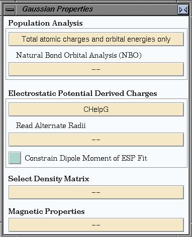
Most importantly, it has a check box that allows you to use the dipole
moment of the molecule as an additional constraint in the ESP calculation.
This is often a good idea. Also, if one method to calculate ESP charges
fails for whatever reason, you can choose a different method here.
Finally, you must select a computer to run the calculations on. Go to the
Job Control window, and select local host. This window
also allows you to se which jobs are running, have finished, etc.
Having one all this, you can hit RUN now, and wait for the result.
importing the QM results
Once your Gaussian calculation has finished, you have to read in the results.
Select Analyze --> Files to read in the Gaussian output. Since you
asked for an ESP calculation, you might think that your molecule now
has the correct charges. But is has not! Select Analyze --> Models to
get the window shown below, that allows you to actually put the ESP charges
on the atoms.
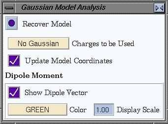
Change No Gaussian into the the correct option, and check that
this actually worked; for example, by labeling the atoms by their charge,
you can see immediately if something changes or not.
Note that the above step is essential to get the correct charges, but is
easily forgotten!
Save the molecule with ESP charges as csp99-2-631gdesp.msi.
Calculating a 'simple' morphology
What will be the morphology of the crystals of our molecule? To answer that
question, we first have to obtain the crystal structure. It has been solved
in 1999, and you can get it
here. The attachement
energy method is a "quick and reasonable" method to predict the crystal's
morphology. It works by calculating the energy between slices in the structure,
as explained in the course. This implies that you should work on optimized
crystal structures. Explain why.
transferring charges
So we first have to optimize the crystal structure. By now, you should know
how to do that. The structure in expII.msi has no charges. Now that's a pity!
There are two ways to put charges on your model. One way is to look at
the charges on your QM model, and enter those into the crystal model. Imagine
doing that on a big molecule, whith hundreds of atoms. So we take another
route.
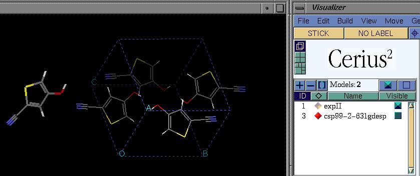
Load the model of the molecule with ESP charges, and also make the crystal
structure visible. Choose the 'overlaid' visualisation mode. Make sure the
ESP model is the active model. Now select all atoms -- this will select all
atoms in the active model. Your screen looks something like this:
By only moving the selected atoms (using CTRL in combination with the
normal mouse buttons) overlay the charges molecule with one of the
molecules in the crystal. Then make a copy of the crystal model, unbuild
the crystal in this model, select the remaining molecule, and delete it.
Don't you end up with an empty model now?? No, you do not. The crystal
information (cell parameters, space group) is still there. Copy the ESP
charged molecule into this 'empty' model, and hit BUILD CRYSTAL.
Voila, you should have your crystal back. Because it has been positioned
according to one of the molecules in the crystal, this structure should be
close to the true crystal, and can be used for optimization. Check this by
comparing the model to the experimental structure.
Save this model
Optimize the structure you just created. It should stay similar to
the experimental structure.
Also save this model
morphology calculation
The OFF INSTRUMENTS 1 card holds the MORPHOLOGY interface.
Hit Calculate and you will get a number of choices for
morphology calculation. Calculate the Growth Morphology using the
default settings except changing Full OFF Support into
Bond-Energy-List. This should speed up the calculations significantly.
The Display window lets you choose what to
visualize: the structure, the morphology, or both, and allows to label the
faces. Labelling by indices is of course quite useful.
Which are the largest surfaces? What does that imply about
the growth speed?
Creating crystal surface models
Let's look at a surface in more detail. For example, what does the 011 surface
look like?
To create a surface hkl, Cerius has the SURFACE BUILDER card in
the card deck, under BUILDERS 1. Creating a surface is called
cleaving in Cerius lingo. Go to the surface builder, and hit Cleave
Crystal Surface. The surface will be built in a new model space, so you
should create one by clicking the  button. In the Cleave window, select the crystal structure you want to build
a surface from.
button. In the Cleave window, select the crystal structure you want to build
a surface from.
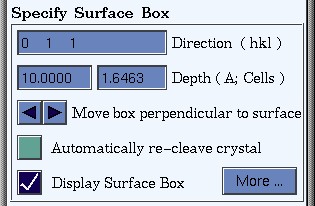
In the Cleave Crystal Surface window, now set the miller indices
of the surface you want to create (0 1 1), and the depth of the surface,
for example 10.0A. This will create a periodic slab of 10A thick, in the 011
direction of the crystal. This 2-D periodic slab consists of surface unit
cells, referred to as "Surface Box" in Cerius.
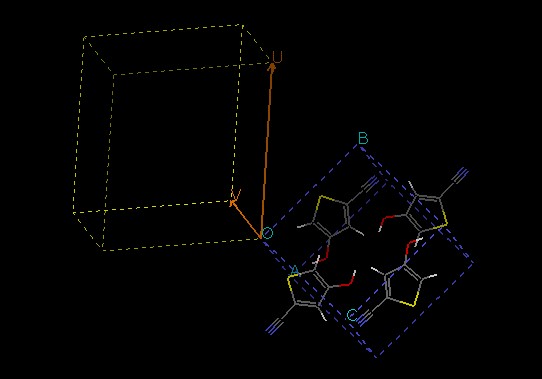
Because you must select/create an empty model space to build the surface in,
you are now staring at an empty model window now. To see what you are
actually doing, also make the structure which is to be cleaved visible, and
overlay it with the empty model space. By switching on Display Surface
Box, you can see which part of the structure will be used as the
surface unit cell. Below is a picture of what the model window should look
like:
What the surface looks like (which atoms or molecules are at the surface)
is not only determined by the orientation of the surface, but can also depend
on the position of the plane which cuts the crystal. For example, if a
structure consists of a stacking of A and B layers, a surface parallel to
those layers may consist of an A layer, or a B layer, depending on where the
crystal was cleaved. If you (think you) know what the surface should look
like, you may have to position the cleavage plane accordingly.
If necessary, you can move the surface box to determine which atoms or
molecule are at the surface, but in this case that will not change
the surface you get. Why?
Hit CLEAVE to create the surface in the empty model space. Make the
model of the original crystal not-visible again (click the 'diamond'). Now
you have a model of the surface unit cell, which you can save in msi format.
Save this model
By just looking at the model you just created, some characteristics of the
011 surface are clear already. Name (at least) one
important feature of this surface
Interaction between surface and solvent
Will 011 have a strong interaction with solvents, like e.g. methanol?
To investigate that, lets put methanol near the surface. Methanol,
with 6-31gd-ESP charges on it, can be downloaded
here.
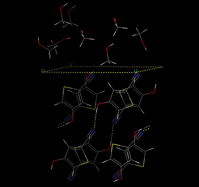
Put some (some=8) methanol molecules near the surface, and make sure they
do not overlap with each other or surface atoms. Save the resulting model,
or at least make a copy in cerius and use that for further calculations; one
mistake, and your model will be ruined! Your model now looks somewhat like
this:
We want to do molecular dynamics on this system, but it is a good idea
to get a reasonable starting geometry first by doing an energy minimization.
Load the Dreiding force field, and, for the time being, use a cut-off
for the non-bonded interactions (i.e. do not use Ewald summation), to speed
up the calculations at this stage.
Also, fix the cell parameters and atomic positions of the molecules in the
crystal (-surface). Those have reasonable postions anyway. To do so, use the
Constraints --> | Atoms/Cell options in the Minimizer card.
Hit minimize, and see what happens. Make a copy of the minimized model.
Sometimes molecules move 'to the next unit cell'. To replace them by a
copy in the original cell (remember we use periodic boundary conditions),
go to the surface bulder again and hit BUILD SURFACE in the
Building From Atoms window. This will move molecules back to a position
on the surface cell.
molecular dynamics The molecular dynamics engine can be found under
the OFF METHODS card, as DYNAMICS SIMULATION. Click Run
to get the window which allows you to set several parameters. What should our
simulation look like?
- Since the size of the surface unit cell is more or less fixed by the bulk
of the crystal, it can be kept constant. Therefore, we will work at constant
volume (as opposed to constant pressure).
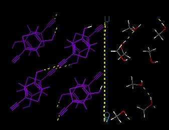
- In our current model, all atoms in the crystal are kept fixed at their
current position. This is a reasonable first approximation, except for the
hydroxyl hydrogens at the surface; the OH group will certainly rotate. This
can be achieved by going to the MINIMIZER card, clicking
Constraints -->, selecting the two hydrogens at the surface, and
clicking Allow Atomic Motion. To check the result, this window also has
a button to Color Atoms by Constraint. Colors should look like shown
here:
- The temperature should be set to some reasonable value. Leave it as is,
at 300K (sort of room temperature). It should be kept at that value during the
simulation, so click CONSTANT NVT.
- The length of the simulation is now 500 steps of 1 fs (0.001 ps), i.e.
0.5 ps. This is very short. For a start, set the number of steps to 5000, so
the run will be 5 ps.
- Save the results of the MD simulation. Each step of dynamics results if new
atomic positions and velocities, and those can be saved during the simulation
in a so called trajectory file. You can find this option in the
Trajectory..., window. Saving just the positions (i.e. not including
the velocities) is enough at this time.
Hit RUN DYNAMICS, and off you go!
MD analysis
The above simulation should take just a few minutes. When it has finished,
the results can be analyzed in a number of ways. Start by reading in the
trajectory, via OFF METHODS | ANALYSIS | Input. Use Show Frames
to "play back" the trajectory. Hydrogen bond formation is one interesting
feature to follow during such a run. Under the Build menu (not card),
go to Edit H-Bonds..., and switch on Enable automated
recalculation. Now, hydrogen bonds wil be calculated for each frame in the
trajectory (if you would just click CALCULATE, H-bonds would be
calculated for the current frame and kept the same for all other frames).
Play back the trajectory.
Describe what you see: how
mobile are different atoms/molecules? Which torsions rotate?
To get a more detailed view of what is going on, variables like total energy
and its components, temperature, or selected angles/distances can be plotted
as a function of time. You can find these options under Analyze -->
Statistics. Left-clicking selects a variable, clicking while pressing
Shift or Control extends the selection. Plot the total, kinetic and potential
energy. What do you see?
This MD simulation was more or less 'quick and dirty': it took only a short
time (CPU time, that is), but it may not be very realistic.
What would you change to the model and the simulation
parameters to get a more reliable result?
simulation of a non-periodic system
Simulations (MM, MD, ...) in Cerius can be 3D-periodic, 2D-periodic, or not
periodic at all, corresponding to crystals or infinite volumes of gas/liquid
(3D), surfaces (2D), or isolated clusters of material. We will now look
at the behaviour of such a 'drop' of material with MD, and simulate the
crystallization of NaCl.
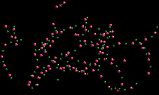
What we want to do is see how NaCl solidifies from a cloud of Na+
and Cl- ions. Start by creating this orderless cloud of some
100 Na+ and 100 Cl- ions. This can be tricky, but
by repeatedly copying and pasting between models, and saving regularly
so you do not loose everything if you make a mistake. Sometimes your
model seems to have disappeared after pasting more ions into it. This is
(probably?) due to scaling by Cerius to avoid overlapping atoms. Move pasted
atoms before you paste the same model again into your final model. Eventually,
you should get a model loke shown here (of course, your NaCl cloud may be
shaped totally differently).
What about the MD simulation parameters? As usual, use the Dreiding
force field, and in this case use a 'direct' cut off (i.e. a single cut off
radius) of 200 A, for van der Waals and Coulomb interactions. This large
cut off radius ensures all ions feel each other. The melting point of NaCl
is 801 C, so if you set the temperature to e.g. 600 K the cloud should
solidify rapidly.
Before running the MD, it is a good idea to perform a few (say, 10) steps
of energy minimization, to get rid of close contacts. Those might mess up
your MD, as they add a giant amount of (potential, later kinetic) energy
to the system.
Run the MD at constant NVT (V is not really defined here, but constant P
would require system dimensions that can be adjusted). It is a good idea
to first do a test run of just a few ps on a copy of the system, to see that
all is working well. Then start a run of ~150 ps. Make sure you save the
trajectory file! By default, it gets written every 10 steps, which would
lead to thousands of frames being saved. Let's not overdo it, and save
one frame in every 100, so the trajectory will contain 1500 frames, one
every 0.1 ps. Carry out the MD run. This should
take about one hour on a modern SGI; it may be helpful to run such a job on
the vstofsgi server, or let it run overnight on an Indy. The analysis of the
results is part of the next part of the course.
Once you have done all this, get back to the
main course page.