Molecular modelling of crystal structures --
part 4
Analysis of simulations, and using scripts
In this excercise, you will analyze the results from MD and other simulations.
MD trajectory analysis
playing back MD movies
Load the trajectory file of the NaCl simulation (OFF METHODS card,
ANALYSIS | Input). Play back the MD movie via the Show Frames
window. Do not be surprised if it takes some time for the movie to actually
start playing: before the MD movie can be displayed, all frames are read
from the trajectory file, which takes some time. The next time you hit the
play button, the movie will start playing immediately.
Describe what you see.
How can we correlate the movie to 'hard numbers'? A plot of the potential
energy vs time can be helpful. Go to Analyze --> | Statistics to
make such a plot. How does this help you? What happens
at what time?
Making plots like you just did can be time-consuming, because your
workstation is probably not very fast, and all data have to be transported
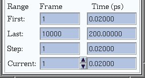
over the network. We can work around this in several ways. Reading (trajectory-)
files is much faster if you are working on the same computer as the data
are stored on. Furthermore, in many cases you do not need all frames that
have been stored. For example, you can read in just one frame in every ten,
or use only frames from a specified time interval. The Input window
holds these options, as show below.
calculating an RDF
A very useful funtion to analyze the NaCl system is the radial
distribution function, or RDF. In essence, the RDF counts
how often two atoms are found at a particular distance from each other. The
result is a histogram, where each bar corresponds to an interatomic distance
interval (e.g. 2.5-2.6 A), and its height shows how often that distance was
found. The height is relative to the value that is to be expected if no
particular ordering would be present in the system, given the density of
particles. So, a value of 1 means "nothing special going on", values
hihger than 1 indicate a preference for a specific distance, and values
below 1 show that atoms avoid that distance.
An RDF can be computed taking into account all atoms, but also a
selection, for example only carbon atoms. The menu to calculate RDF's is
found under Analyze --> | RDF. If the RDF is calculated on an MD
trajectory, for each frame the calculation is done, and the average is plotted.
Calculated the RDF including all atoms of the NaCl MD trajectory. During the
calculation, the shape of the plot slowly changes. What
changes, why, and which peak corresponds to which distance?
Also make an RDF for the Na-Cl distances. Compare the
height of the peaks to those in the previous plot.
The structure changes during the MD run. The RDF's you made so far are an
average of two rather different phases. Select those frames in the trajectory
that correspond to the final phase, and make an RDF using all atoms.
Explain the peak positions and their shapes.
other plots from MD
Let us go back to the MD simulation of methanol on the CSP99-II surface.
We could analyze that run als o via RDF's. Which
interatomic distances could be interesting?
But we won't... Instead, we will look at some geometric parameters.
If you measure a distance/angle/torsion angle in the model,
it can be selected for plotting as a function of time, via the Analyze -->
| Statisctics window. For example, measure one of the H-C-O-H torsion
angles in one of the methanol molecules. Now select it for plotting, and make
the plot. Explain the graph.
Do the same for the hydroxyl groups of the CSP99-2 molecules (of course,
only those at the surface; the others are kept rigid, so the graphs would
be rather boring...). How flexible are these compared
to the methanol hydroxyls?
At the surface, the hydroxyl groups of CSP99-2 have two low-energy positions.
The time spent near each energy minimum will depend on the relative energies
of the minima; vice-versa, in principle we could determine their relative
energies from the time spent in each minimum during the MD run: the probability
to find a conformation depends on E via a Boltzman distribution.
Suppose we would carry out a 40 ps MD run, and examine the conformation of
one of the OH groups. It starts in one conformation, and flips over to
the other position after 20 ps. What can we conclude
from that about the relative energies of the two conformations?
interaction energies
It can be interesting to compare the interaction of one solvent with different
surfaces of the same crystal, or between one surface and different surfaces.
Interaction energies may offer part of the explanation for growth rates.
How can we calculate the interaction between solvent and surface?
Select a frame somewhere half way the MD run. Set up the energy calculation
identical to what was used in the MD simulation. Now, calculated the current
energy of this frame, without minimization. Then, select all solvent molecules,
open the Move | Translate window, and move all selected atoms far
(~50 A) away from the surface. Then, recalculate the current energy.
The difference between the two energy values you just calculated is the
interaction energy for this frame. Explain why.
This energy will fluctuate during the MD simulation, and the average is
probably what you are interested in. This means you have to repeat the above
procedure for many frames. That does not sound like fun, does it. Fortunately,
It is not necessary to do this by hand, because there exists something
like a Cerius scripting language.
Scripts -- using Cerius non-interactively
Cerius can be used interactively, via the graphical interface, but also by
entering text commands on the commandline, or via a set of commands stored
in a file, a so called script. In fact, all commands or actions carried out
during an interactive session are stored in a script: this is the RUN.LOG file
that is there after you quit Cerius. This file is written when you quit
the program; if you want to see the text commands equivalent to your actions
so far without leaving Cerius, look under the Utilities | Record
Commands... menu.
Next to the specific Cerius commands, commands from the scripting language
tcl can be used in scripts. This makes it possible to write
loops, and do other useful things. Two example scripts are shown here.
They can be used from the commandline via the command:
/home/msi/cerius2_4.6/bin/cerius2 -n -o output.out scriptfile.log
You may have to adapt /home/msi/cerius2_4.6/bin/cerius2 to your local
system's settings. the -n option switches off the graphics interface,
-o specifies the file that will hold the text output from the program,
and scriptfile.log is your script, or, in Cerius lingo, log file.
A script to do an MD run may look like this:
############################################################
# Log RUN.LOG created Thu Jan 31 15:40:07 2002
# Cerius2: Version 4.2 MatSci
############################################################
FILES/LOAD "./surf.010-etoh-periodic-3x3.msi"
FORCE-FIELD/LOAD_FORCE_FIELD "././Cerius2-Resources/FORCE-FIELD/DREIDING2.21"
FORCE-FIELD/COULOMB_REAL_CUTOFF 12
FORCE-FIELD/COULOMB_REAL_CUTIN 10
FF_EDITOR/COULOMBIC_FUNCTIONAL_FORM "CONST-EPS"
DYNAMICS/TRAJECTORY_PERIOD 50
DYNAMICS/WRITE_TRAJECTORY YES
DYNAMICS/TRAJECTORY_FILENAME "md-3x3p-300k"
DYNAMICS/RUN_TIME 100000
DYNAMICS/METHOD "CONSTANT NVT"
DYNAMICS/RUN_SIMULATION
############################################################
# Log closed Thu Jan 31 15:42:57 2002
############################################################
All lines starting with # are comments, and will be ignored by Cerius.
The commands are rather self-explaining: a model file is read, the force field
is loaded and the cut offs set, MD parameters are set and the simulation is
started. Another example: the calculation of interaction energy between
solvent and surface for a set of frames from an MD run:
############################################################
FORCE-FIELD/LOAD_FORCE_FIELD ././Cerius2-Resources/FORCE-FIELD/DREIDING2.21
FORCE-FIELD/COULOMB_REAL_CUTOFF 12
FORCE-FIELD/COULOMB_REAL_CUTIN 10
FF_EDITOR/COULOMBIC_FUNCTIONAL_FORM CONST-EPS
############################################################
MD_ANALYSIS/TRAJECTORY "./md0_10bflex.trj"
MD_ANALYSIS/CURRENT_FRAME_NUMBER 1
MECHANICS/AUTOSET_VARY_CELL NO
############################################################
#Scriptfile processing completed
SELECT/DESELECT_ALL -SCOPE "ALL MODELS"
SELECT/RULE ADD
SELECT/CRITERION -TOOLBAR Frag
SELECT/FRAGMENT RESTART Cell(0,0):Atom(1850)
SELECT/FRAGMENT TOGGLE Cell(0,0):Atom(2000)
SELECT/FRAGMENT TOGGLE Cell(0,0):Atom(2150)
SELECT/FRAGMENT TOGGLE Cell(0,0):Atom(2300)
SELECT/FRAGMENT TOGGLE Cell(0,0):Atom(1250)
SELECT/FRAGMENT TOGGLE Cell(0,0):Atom(1400)
SELECT/FRAGMENT TOGGLE Cell(0,0):Atom(1550)
SELECT/FRAGMENT TOGGLE Cell(0,0):Atom(1700)
SELECT/FRAGMENT TOGGLE Cell(0,0):Atom(650)
SELECT/FRAGMENT TOGGLE Cell(0,0):Atom(800)
SELECT/FRAGMENT TOGGLE Cell(0,0):Atom(202)
SELECT/FRAGMENT TOGGLE Cell(0,0):Atom(52)
SELECT/RULE TOGGLE
SELECT/ALL
SELECT/RULE RESTART
for {set i 20 } {$i < 2001} {incr i} {
set framenr [expr 1*$i]
MD_ANALYSIS/CURRENT_FRAME_NUMBER $framenr
MECHANICS/CURRENT_ENERGY
MOVE/TRANSLATION_VECTOR 1 0 0
MOVE/TRANSLATION_STEP_SIZE 40
MOVE/AXIS_TRANSLATE - START
MOVE/AXIS_TRANSLATE - END
MECHANICS/CURRENT_ENERGY
}
Here, the energy calculation is set up, a trajectory file is read and the
first frame is taken. Then, all molecules in the crystal are selected, and
this selection is then inverted, so only the solvent molecules are selected.
This is simpler to do then selecting all solvent molecules, because there
are so many of those in this case. In the loop, which starts at the line
for {set i 20 } etc... a frame is read, the energy is calculated, all
selected atoms (in this case: the solvent) are translated, and the energy is
calculated again.
The output of the above scripts will be written to the terminal window, or
can be sent to an output file. To get the interaction energies from that file,
you will need to browse through it, or, if you are a conaisseur, you can write
a UNIX script to do so for you. Try grep " Total Energy :" outputfile
for example.
A practical way to create Cerius scripts is to carry out the necessary
actions in the GUI, quit Cerius, and then rename and edit the logfile. If
you plan to do MD runs on the same system at 5 different temperatures
for example, this is a good approach: create one logfile, and make
several scripts from it by copying and just changing the temperature.
You can also execute scripts from the GUI: see Utilities | Playback
Script.... This can be a quick way to perform standard actions, like
setting graphics parameters.
Create a script that makes a copy of the current
model, overlays the copy with the original and does a geometry optimization
onthe copied structure.
This is the end of the Cerius hands-on course. If you attended the
'caput college', worked through the five parts of the course and hand in
your answers to the questions, you may be entitled to 3 study points.
Back to the main course page.